How to Calculate a P-Value from a T Test

Hands calculating p-value with calculator

The p-value from a t test is the probability, under the Student's t distribution, of observing a t statistic at least as extreme as yours if the null hypothesis were true. For a two-tailed test, the formula is:

p = 2 × CDF_t(df)(−|t|)

For a one-tailed test, it's either CDF_t(df)(t) for a left-tailed test or 1 − CDF_t(df)(t) for a right-tailed test. The shape of that CDF depends entirely on your degrees of freedom.

One-line verification snippets for the three tools researchers reach for most:

R: 2*pt(-abs(t), df)
Python (SciPy): from scipy import stats; p = stats.t.sf(abs(t), df)*2
Excel (two-tailed): =T.DIST.2T(ABS(t),df)

The p-value does not tell you the probability that your null hypothesis is true. It tells you how often you'd see data this extreme if the null were true. That distinction shapes every decision you make downstream.

Gostellar's resources on p-value interpretation are a useful companion if you want the conceptual framing alongside the mechanics covered here.

Key Takeaways

The most reliable t test p value calculation uses 2*pt(-abs(t), df) in R or stats.t.sf(abs(t), df)*2 in Python, always with the absolute value of t and the correct degrees of freedom.

Point	Details
Two-tailed formula	p = 2 × CDF_t(df)(−
Degrees of freedom	One-sample: n−1; paired: n_pairs−1; independent equal-variance: n₁+n₂−2.
Software cross-check	Verify every p with a second tool; R, Excel, and GraphPad should return identical values.
T-table gives a range	Tables bracket p between two α levels; use software when exact p is required for publication.
Report more than p	Always pair p with effect size (Cohen's d) and a 95% CI for a complete result.

Step-by-step worked example: from sample stats to p-value
How to read a t-table when you don't have software
Exact p-value recipes for R, Python, Excel, and online calculators
Which tail to use, and how to compute degrees of freedom
Common mistakes that produce wrong p-values
When t-test p-values can mislead you
A recommended workflow for trustworthy p-value reporting
Sources

Step-by-step worked example: from sample stats to p-value

Walk through this once by hand and the formula stops feeling abstract.

The setup: You measure resting heart rate in a sample of n = 25 adults. Your sample mean is x̄ = 72.3 bpm, the sample standard deviation is s = 8.1 bpm, and you want to test whether the population mean differs from μ₀ = 70 bpm (two-tailed, α = 0.05).

Step 1: Compute the t statistic.

The one-sample t formula is:

t = (x̄ − μ₀) / (s / √n)

Plugging in: t = (72.3 − 70) / (8.1 / √25) = 2.3 / (8.1 / 5) = 2.3 / 1.62, which calculates to a bit above 1.4

Degrees of freedom: df = n − 1.

Step 2: Locate the t statistic on the distribution.

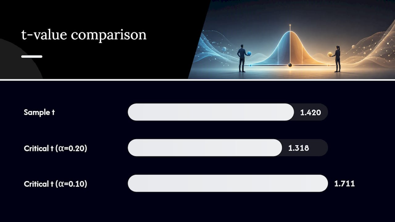
The t distribution with df = 24 is bell-shaped but heavier-tailed than a normal. Your t = 1.420 sits in the right tail. For a two-tailed test, you want the combined probability in both tails beyond ±1.420.

Student's t distribution curve with tails shaded

Step 3: Estimate from a t-table.

Looking at a standard t-table for df = 24, the critical values are approximately t = 1.318 (α = 0.20 two-tailed) and t = 1.711 (α = 0.10 two-tailed). Your t = 1.420 falls between those, so p is between 0.10 and 0.20.

Step 4: Get the exact p-value with software.

R: 2*pt(-abs(1.420), 24) → p ≈ 0.1685
Python: stats.t.sf(abs(1.420), 24)*2 → p ≈ 0.1685
Excel: =T.DIST.2T(ABS(1.420),24) → p ≈ 0.1685

p ≈ 0.1685 is well above α = 0.05, so you fail to reject the null. For a sharper reference point: Statistics By Jim demonstrates a comparable worked example where t = 2.289 with df = 24 yields a two-tailed p just below 0.05, indicating statistical significance.

Step 5: Report the result.

Write it as: t(24) = 1.420, p = 0.169 (two-tailed). Always include df, the exact p, and the tail specification. Statology's step-by-step guide reinforces this sequence and is worth bookmarking for quick reference.

How to read a t-table when you don't have software

Printed t-tables give you a p-range, not an exact value. That's usually enough to make a significance decision, and knowing how to use them keeps you from being helpless without a computer.

How the table is organized. Rows correspond to degrees of freedom. Columns correspond to critical t values for specific two-tailed α levels (commonly 0.20, 0.10, 0.05, 0.02, 0.01). Each cell shows the t value you'd need to reach that α. Khan Academy's video walkthrough maps this visually if you prefer seeing the tail areas shaded.

The lookup process. Go to the row for your df. Scan across the columns to find where your |t| falls. If |t| = 1.420 with df = 24 sits between the columns for α = 0.20 and α = 0.10, you report p ∈ (0.10, 0.20). That's your range.

Pro Tip: Always use |t|, not the signed value. If your df isn't listed as an exact row, use the next smaller df available. This gives a slightly conservative (larger) p-range, which is the safer direction for a significance decision.

One practical limit: tables typically stop at df = 30 or df = 40 and then jump to ∞. For df between listed rows, the conservative approach keeps you from overstating significance. When precision matters for publication, always verify with software.

How to read a t-table when you don't have software — overview diagram

Exact p-value recipes for R, Python, Excel, and online calculators

R

t_stat <- 1.420
df     <- 24

# Two-tailed
p_two  <- 2 * pt(-abs(t_stat), df)

# Left-tailed
p_left <- pt(t_stat, df)

# Right-tailed
p_right <- pt(t_stat, df, lower.tail = FALSE)

The key argument is lower.tail = FALSE, which gives the survival function directly. The distributions3 R reference documents pt() arguments precisely and explains why passing a negative absolute value (-abs(t)) is the safest pattern for two-tailed tests.

Python (SciPy)

from scipy import stats

t_stat = 1.420
df     = 24

# Two-tailed
p_two   = stats.t.sf(abs(t_stat), df) * 2

# Left-tailed
p_left  = stats.t.cdf(t_stat, df)

# Right-tailed
p_right = stats.t.sf(t_stat, df)

stats.t.sf is the survival function (1 − CDF). Using sf instead of 1 - cdf avoids floating-point precision loss when p is very small, which matters when you're working with extreme t values.

Microsoft Excel

OmniCalculator's documentation covers these Excel functions in detail:

Left-tailed: =T.DIST(t, df, TRUE)
Right-tailed: =T.DIST.RT(t, df)
Two-tailed: =T.DIST.2T(ABS(t), df)

For the worked example: =T.DIST.2T(ABS(1.420),24) returns 0.1685. Note that T.DIST.2T requires a non-negative t value, so wrapping in ABS() is mandatory.

Online calculators

GraphPad's p-value calculator accepts t and df directly and returns the exact two-tailed p alongside a 95% confidence interval. It also notes that positive and negative t values produce identical p-values.
Social Science Statistics offers separate left-, right-, and two-tailed calculators, useful for classroom work.

Verification across tools for t = 1.420, df = 24:

Minor rounding differences (e.g., 0.168 vs. 0.1685) appear when you round the t statistic before passing it to the function. Always carry full decimal precision through the calculation.

Which tail to use, and how to compute degrees of freedom

Choosing your tail

Your alternative hypothesis determines the tail, not your data:

Two-tailed (H₁: μ ≠ μ₀): Use T.DIST.2T or multiply the one-tailed p by 2. This is the default for most research contexts.
Left-tailed (H₁: μ < μ₀): Use T.DIST(t, df, TRUE) in Excel or stats.t.cdf(t, df) in Python.
Right-tailed (H₁: μ > μ₀): Use T.DIST.RT(t, df) in Excel or stats.t.sf(t, df) in Python.

Choosing a one-tailed test because your observed t happened to go in the "right" direction is p-hacking. The tail must be specified before you see the data. Gostellar's guide on one-tailed vs. two-tailed tests covers this decision in the A/B testing context specifically.

Degrees of freedom by test type

One-sample t-test: df = n − 1
Paired t-test: df = n_pairs − 1 (treat the differences as a single sample)
Independent two-sample t-test (equal variances assumed): df = n₁ + n₂ − 2
Welch's t-test (unequal variances): df is estimated by the Welch-Satterthwaite equation; let your software compute it rather than doing it by hand

Quick checklist before you compute p:

Confirmed whether observations are paired or independent
Used the correct n (pairs, not total observations, for a paired test)
Verified variance assumption (equal vs. unequal) for two-sample tests
Noted df explicitly so it can be reported alongside p

Common mistakes that produce wrong p-values

These errors show up constantly, even in published work.

Forgetting abs(t). Passing a negative t to a right-tail function returns p > 1. The distributions3 documentation flags this explicitly. Always use abs(t) or -abs(t) depending on the function.
Using dt instead of pt in R. dt is the density function (the height of the curve), not the CDF. It returns a probability density, not a tail probability. A community thread on StackExchange documents this exact confusion with concrete examples.
Not doubling for a two-tailed test. pt(-abs(t), df) gives one tail. Multiply by 2 for a two-tailed p.
Wrong df. Using n instead of n − 1, or forgetting to use n_pairs for a paired test, shifts the distribution and changes p.
Sign errors in Excel. T.DIST.RT requires a positive t. Passing a negative value gives the wrong tail.

Validation checklist when a p-value looks suspicious:

p > 1 or p < 0: you passed the wrong sign or used the density function instead of the CDF
p = exactly 0.5: you likely passed t = 0 or forgot abs()
p is much smaller than expected: check df; a much larger df than intended compresses the tails
Cross-check with a second tool (e.g., R result vs. GraphPad)
Confirm the t-table range brackets your exact p (if p = 0.003 but the table says p > 0.05 for your t and df, something is wrong)

Minitab's manual p-value documentation also walks through lower-, upper-, and two-tailed cases with explicit CDF steps, which is useful when you're tracing a discrepancy.

When t-test p-values can mislead you

A p-value below 0.05 does not mean your effect is large, practically meaningful, or that the null hypothesis is false. Investopedia's overview puts it plainly: p is the probability of obtaining data at least as extreme as observed under H₀, nothing more.

Three practical checks every experimenter should run alongside p:

Report effect size. Cohen's d for t-tests gives you the magnitude of the difference in standard deviation units. A p = 0.04 with d = 0.08 is a statistically detectable but practically negligible effect.
Report confidence intervals. A 95% CI that barely excludes zero tells a different story than one centered far from zero. CIs communicate both direction and precision.
Pre-register your hypothesis and tail. Deciding on a two-tailed test after seeing a trend toward one direction inflates your false-positive rate.

For A/B testers specifically, sequential testing methods and Bayesian approaches can be more appropriate than a fixed-sample t-test, particularly when you're peeking at results before the sample is complete. Gostellar's guide to A/B test significance covers these practical tradeoffs in a marketing context.

A recommended workflow for trustworthy p-value reporting

The steps below are short, but skipping any one of them is where errors creep in.

1. Compute t with the correct formula. Write out the formula explicitly: one-sample, paired, or independent. Confirm n, s, and the null value before plugging in.

2. Pass abs(t) to your CDF or survival function. This single habit eliminates the most common coding error. Use 2*pt(-abs(t), df) in R or stats.t.sf(abs(t), df)*2 in Python.

3. Verify with a second tool. Run the same t and df through GraphPad or Social Science Statistics. If the two results differ by more than rounding, trace the discrepancy before reporting.

**4. This gives readers everything they need to evaluate your result.

5. Document df, tail, and method. Note whether you assumed equal variances (Student's) or not (Welch's), which tail you used and why, and which software version produced the result. Reproducibility depends on these details.

Sources

Use these resources for exact calculations, deeper learning, and quick verification:

Try Stellar A/B Testing for Free!